**************************************************************************************************************
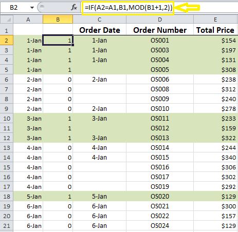
*******************************************Welcome to Blog post #100***************************************** *************************************************************************************************************** During the past three weeks, I demonstrated how to highlight alternate data groupings in MS Excel and also how to address blanks in doing so. This week I will show how to calculate and return the sum of values in alternate data groupings. STEP 1]Create the two helper columns as explained in my last blog post. I have placed them in columns A and B this time.
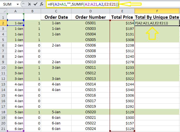
STEP 2] Use the following formula to sum alternate groupings.
=IF(A2=A1,"",SUMIF(A2:A21,A2,E2:E21))
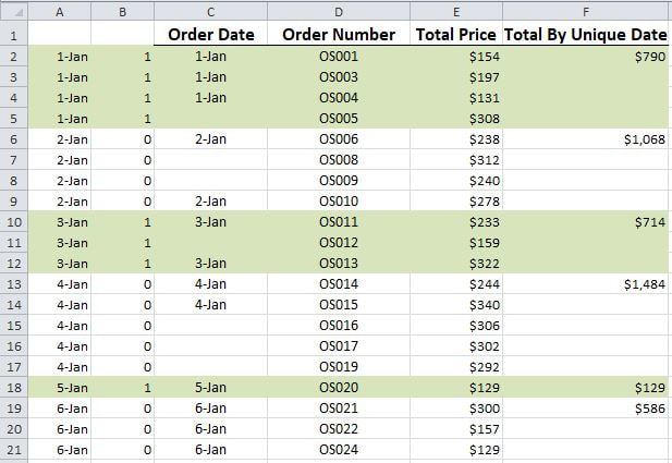
Here is the final desired outcome after the formula has been applied to the entire range.
0 Comments
|
CategoriesArchives
June 2020
|


