|
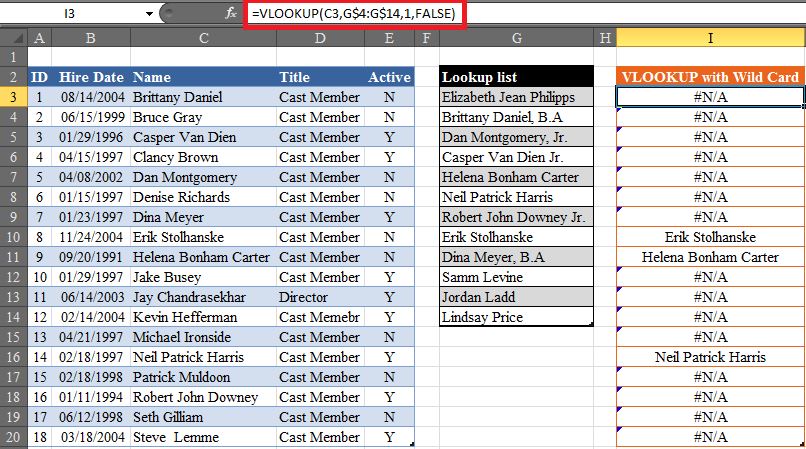
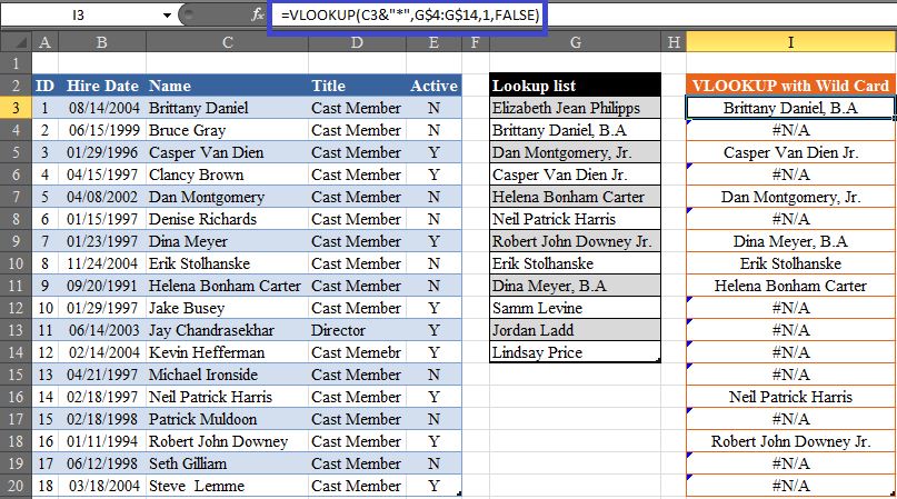
The purpose of this blog post is to illustrate how to use a wildcard within a VLOOKUP. Doing so will allow the VLOOKUP formula to not only return exact matches between the lookup value and the lookup list (as a conventional VLOOKUP does), but to also when required return values when there is a partial match. I will illustrate this using a tangible example. As you could see in the VLOOKUP column in the table below, I have used a VLOOKUP in order to find matches between the lookup list (I.e. Values in Column G) and the lookup values (I.e. Values in Column C), However; since the lookup values don’t have suffixes (e.g. B.A, Jr.) some of their respective matches in the lookup list which do contain such suffixes are not being returned by the VLOOKUP. In the example above, it is clearly evident that the values for many matches have not been returned because of the suffix that is attached to the name in the lookup list. Here is the list of individuals who didn't appear in the result of the VLOOKUP. · Brittany Daniel, B.A · Dan Montgomery, Jr · Casper Van Dien Jr. · Robert John Downey Jr, · Dina Meyer, B.A It can be clearly observed that all these values have a suffix at the end of the full name. In order to avoid this problem the best solution is to use a wildcard within the VLOOKUP. Wildcard characters are supported in the VLOOKUP function when a text string is used as the lookup value and the last argument in the VLOOKUP indicates exact logic (either FALSE or 0). There are two wildcards to choose from: 1. The “?” wildcard will match any single character 2. The “*” wildcard will match any number of characters. Here is the formula I will be using to fix the dilemma: =VLOOKUP(C3&"*",G$4:G$14,1,FALSE) For example, the value for “Robert John Downey” would match the value for “Robert John Downey Jr.” Here is the formula in practice:
0 Comments
|
CategoriesArchives
June 2020
|


