|
The conditional formatting feature of MS excel enables us to create a Gantt charts very similar to a MS project Gantt chart. Consider the table below demonstrating a subset of the testing activities that need to be performed during a software testing cycle of a project.
Using the five steps explained below we could create a Gantt chart based on the start and end sates for each of the testing periods.
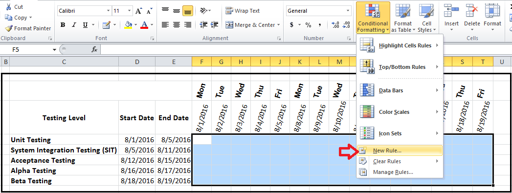
STEP 1] First select the range of cells that you would like conditional formatting to be applied to and then go to the home tab of the ribbon, select “Conditional Formatting” and click on “New Rule”.
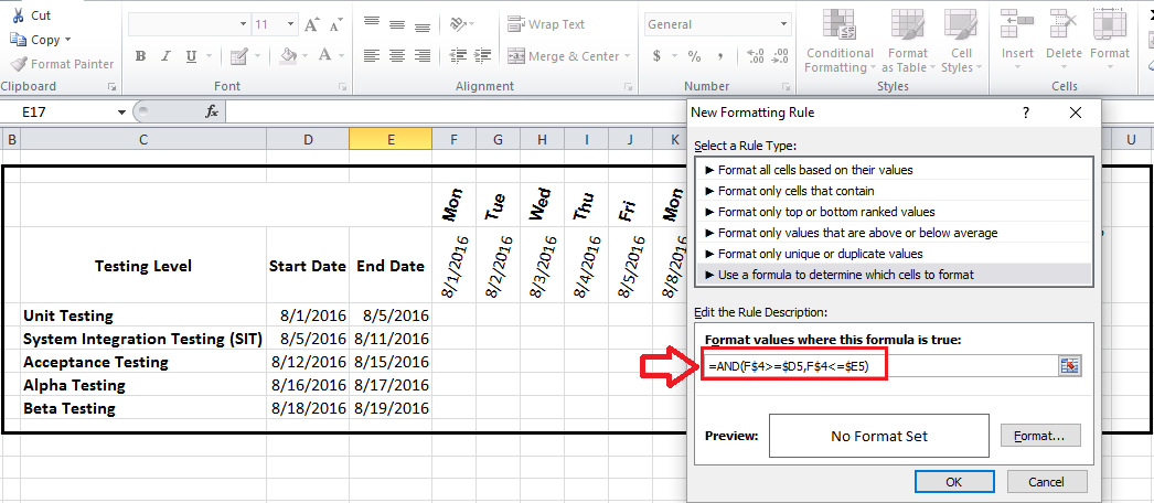
STEP 2] Enter a formula similar to the one below. After inputting the formula, click on “Format” and proceed to step 3.
How does this formula work?
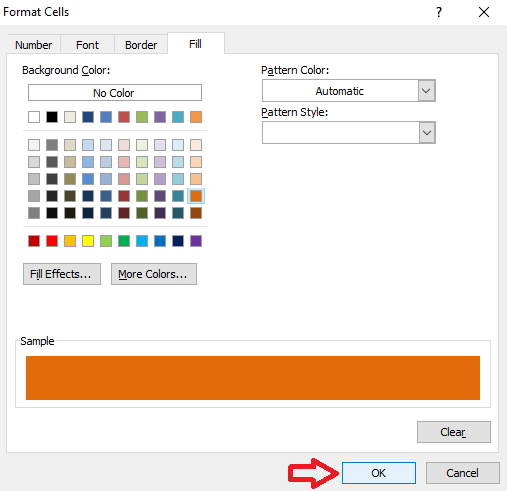
=AND(F$4>=$D5, F$4<=$E5) This formula basically provides a value of true whenever the dates located on row four, fall between the respective Start Date and End Date for each phase. Note that in the formula above it is require to reference lock the values using the $ sign so that the correct range is applied. For example, the $ in F$4 creates a horizontal reference lock and the $ before D5 (I.e. $D5) creates a vertical reference lock. STEP 3] in the “Fill” section chose a color of your choice and click on “OK”
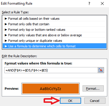
STEP 4] Click on “Ok” a second time.
STEP 5] Here is the desired Gantt chart
0 Comments
|
CategoriesArchives
June 2020
|


