Most of us are used to having fixed lookup values in the lookup field of a VLOOKUP statement. The traditional VLOOKUP does not have dynamic lookup fields. In this blog post, I will demonstrate with example how to write a VLOOKUP statement with dynamic “drop down filter-based” lookup values.
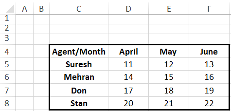
Consider the table below containing a list of agents and their respective sales figures for the months of April, May, and June.
In the screenshot below I have created two drop down filters: one for “Agent” and the other for “Month”. The values for “Agent” are linked to column C (Cells C5 to C8) and the values for “Month” are linked to row 4 (Cells D4 to F4).
Now I want to create a VLOOKUP that uses the dynamic values of “Agent” and “Month” as the lookup values.
Here is the formula I will use for this purpose: =VLOOKUP(I4,C5:F8,MATCH(I5,C4:F4,0),0)
How this formula works?
This formula is similar to a normal VLOOKUP, the only difference is that the instead of inserting a number in the “index number” section of the VLOOKUP, I have used the “Match” formula. The Match formula uses the C4 to F4 range as the lookup array. This way it could return the respective value for either April (i.e. Value in column D), May (i.e. Value in column E) or June (I.e. Value in column F). Note that the MATCH(C4:F4) deliberately includes the C4 value (as oppose to starting from D4) so that the number returned is in sync with the table used by the VLOOKUP. Now let’s test the VLOOKUP statement: I will use “Don” and “June” as the respective values from the “Agent” and “Month” filter values. As per the screenshot below the desired outcome has been achieved from the VLOOKUP statement:
0 Comments
|
CategoriesArchives
June 2020
|


