
A slicer is a visual way to filter your data in pivot tables. A slicer could be added though the insert section of the ribbon. Note: you need to have Excel 2013 or later versions to add a slicer as this feature is relatively new and did not exist in earlier versions of MS Excel.
Consider the data set below containing seven fields. Let’s say we want to create a slicer for the “Region” field (i.e. Central, North, East, and West). 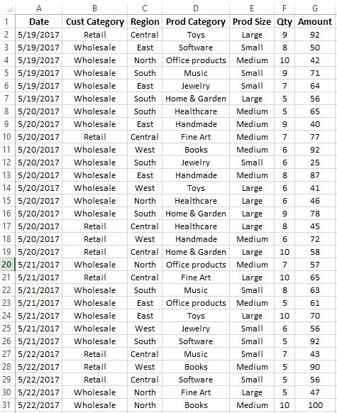
Here are the steps that need to be taken to create this slicer:
STEP 1] Create a pivot table on the data set. 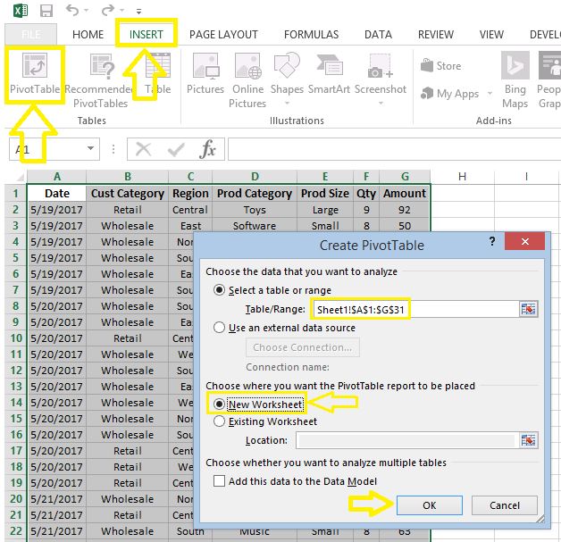
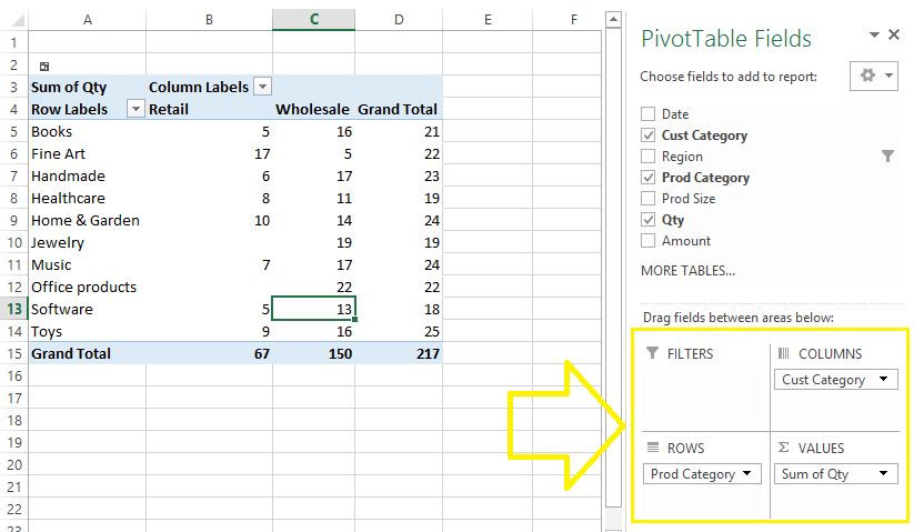
STEP 2] Indicate the desired pivot table fields.
STEP 3] Left click on any cell of the pivot table and go to “Insert” > “Slicer”.
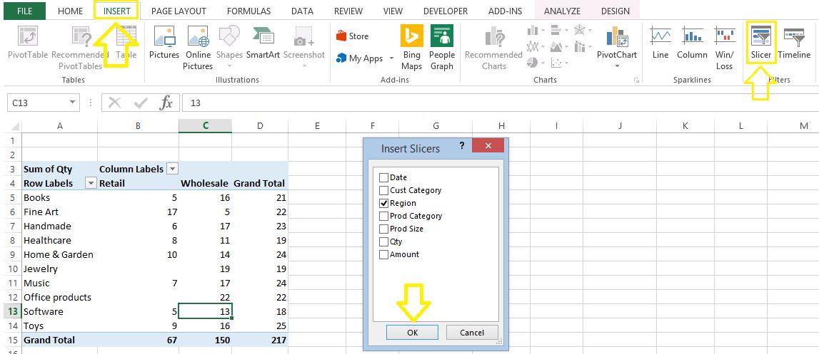
STEP 4] tick the box for which you want to create the slicer (In the case of this example “Region”) as depicted above. Then click on “OK”.
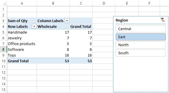
The slicer has been successfully created. By clicking on each of the four buttons on the slicer, the cumulative data for only that one region alone will be displayed.
0 Comments
|
