WISDOMBYDATA
  • BLOG
    • Blog Guide
    • Blog History
  • EXCEL
    • Functions & Formulas
    • VBA & Macros
    • VLOOKUP
    • Pivot Tables
    • Conditional Formatting
    • Tricks & Shortcuts
  • BI
    • SAP BOBJ/BW
    • Tableau
  • SQL
  • ABOUT
    • About WBD
    • About Me

Sum cells in MS Excel based on background color

4/30/2016

2 Comments


The VBA feature of MS Excel makes it possible to sum cells based on their background color. Summing cells based on background color could save lots of time and add a lot of value to the task at hand.
Consider the example below. 
Picture
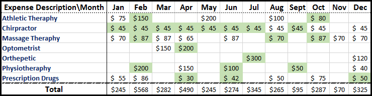
The table above demonstrates all annual healthcare expenses for an individual. The cells that have a light green back ground color are the expenses that the individual paid themselves but eventually got reimbursed for by their insurance firm. As you could see the last row of the table sums up all expenses for each month irregardless of the background color of the cells. 

Here are four simple steps that would allow us to do the sum based on the background of the cells so that we could know how much of the expenses have been covered by insurance and what amount hasn’t.

1. Go to the "Developer" tab and left click on “Visual Basic”. If your developer tab is not visible click here to learn how to activate it.
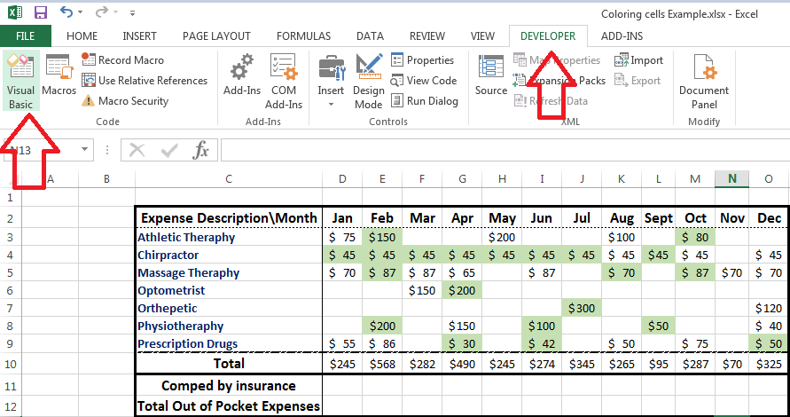
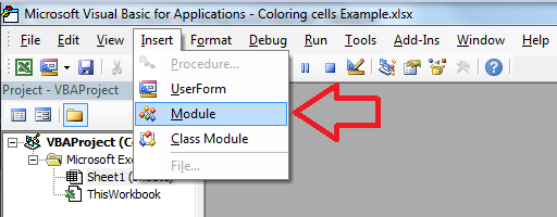
Picture
2. ​While at the VBA screen, select “Insert” and the left click on “Module”
Picture
3. Copy and paste the code below in the code screen:
​
​Function SumByColor(CellColor As Range, rRange As Range)
Dim cSum As Long
Dim ColIndex As Integer
ColIndex = CellColor.Interior.ColorIndex
For Each cl In rRange
    If cl.Interior.ColorIndex = ColIndex Then
        cSum = WorksheetFunction.Sum(cl, cSum)
    End If
Next cl
SumByColor = cSum
End Function
Picture
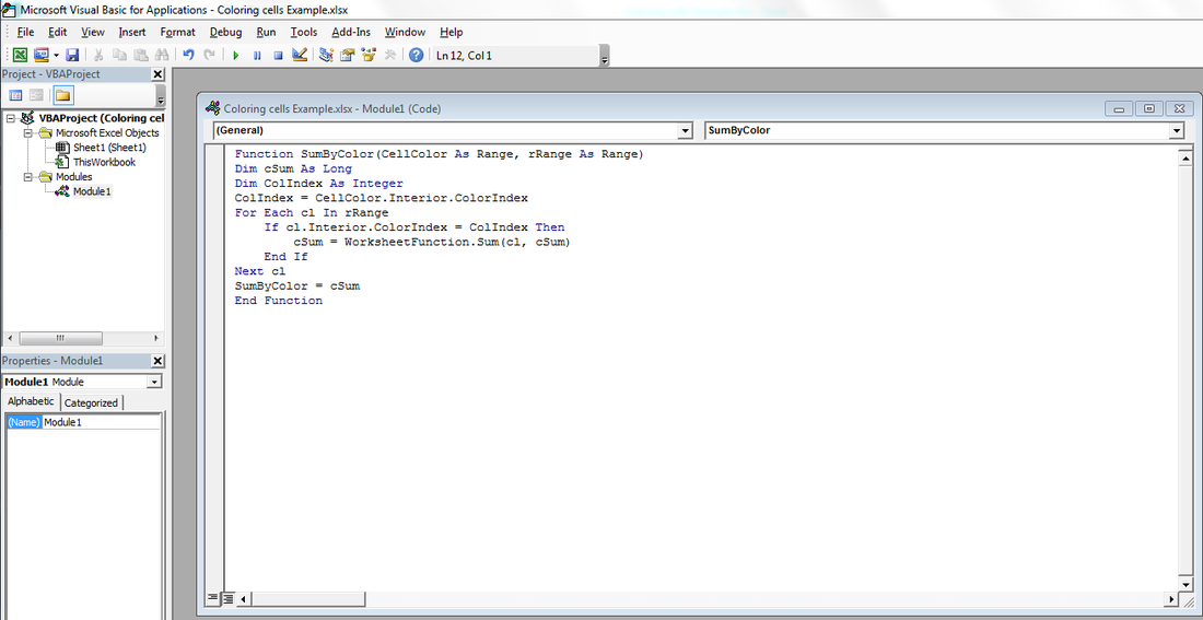
4. Return to the excel tab and type the following formula. and try using the "SumByColor" formula as demonstrates below:
Picture
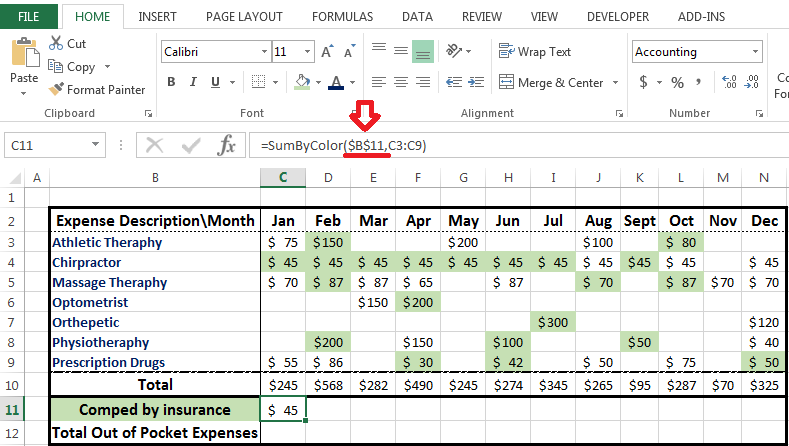
In the screenshot above the SumByColor formula is activated and the first cell used in the formula is a reference to the background color that you wish to be summed. I chose cell $B$11 as the reference. the purpose of the dollar sign ($) is so that the reference wouldn't change after dragging the formula to other cells. As you could see the only amount that has been summed for the month of January using the SumByColor sum statement is the amount that has the light green background color. 

​Here is how the table would look like once the formula is applied for all 12 months.
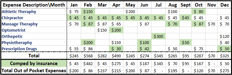
Picture

2 Comments
Sheikh
6/5/2018 08:43:10 am

can this formula be extended on visible cells only. suppose if we filter and can it still sumbycolor.

Reply
Mehran link
6/5/2018 03:50:35 pm

Hi Sheikh,

Thanks for the message. You have raised a very interesting point. I did some investigation on how to return visible colored cells (i.e. visible after applying a filter). It wasn't an easy task at all. I first attempted to combine the SumbyColor function with the SUBTOTAL formula but that didn't work. Then I tried to add the following code to the range of data:

.SpecialCells(xlCellTypeVisible)

That didn't return the desired outcome either. After some research on the web, I finally found the solution! You must create two separate VBA codes in two separate modules: One for "returning visible cells" and the second for "returning cells which are colored". After creating those two VBAs use a formula such as the one below to return the desired outcome:

=SUMPRODUCT(CellsAreVisible(F2:F4,TRUE), CellHasColor(F2:F4,3, FALSE),F2:F4)


I found this solution from the following website:

https://www.excelbanter.com/excel-discussion-misc-queries/168861-subtotal-colored-cells.html

Scroll to near the bottom of the page (i.e. comment by Microsoft MVP: "Chip Pearson"). Both VBA codes are provided there. I have tested this on a sample data set and it INDEED WORKED!!! It was awesome!

I will create a separate blog post in upcoming months demonstrating with example detailed steps that need to be taken to get this task done. But for now this website should provide you with the desired outcome you are looking for.

Thanks again for your productive comment.

Keep visiting for more cool tricks!

Cheers!

Mehran

Reply

Your comment will be posted after it is approved.


Leave a Reply.

    Categories

    All
    BI
    EXCEL
    MISC
    SQL

    Archives

    June 2020
    May 2020
    April 2020
    March 2020
    February 2020
    December 2019
    November 2019
    October 2019
    September 2019
    August 2019
    July 2019
    June 2019
    May 2019
    April 2019
    March 2019
    February 2019
    January 2019
    December 2018
    November 2018
    October 2018
    September 2018
    August 2018
    July 2018
    June 2018
    May 2018
    April 2018
    March 2018
    September 2017
    August 2017
    July 2017
    June 2017
    May 2017
    April 2017
    March 2017
    February 2017
    January 2017
    December 2016
    November 2016
    October 2016
    September 2016
    August 2016
    July 2016
    June 2016
    May 2016
    April 2016
    March 2016
    February 2016
    May 2015
    April 2015
    March 2015
    February 2015
    January 2015
    December 2014
    November 2014
    October 2014
    September 2014
    August 2014
    April 2014
    March 2014
    February 2014
    January 2014
    December 2013
    November 2013

Powered by Create your own unique website with customizable templates.
  • BLOG
    • Blog Guide
    • Blog History
  • EXCEL
    • Functions & Formulas
    • VBA & Macros
    • VLOOKUP
    • Pivot Tables
    • Conditional Formatting
    • Tricks & Shortcuts
  • BI
    • SAP BOBJ/BW
    • Tableau
  • SQL
  • ABOUT
    • About WBD
    • About Me