Calculating Seniority of Active Employees Using MS Excel

---

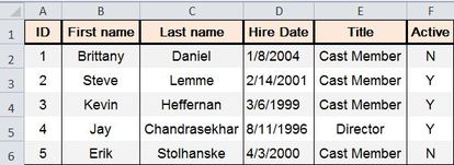
I was assigned the task of creating a report that calculates employee seniority some time ago at work. I was able to use various features of MS Excel in order to perform this task. I would like to share this procedure with you. 
​
Note: the data in the table below are doctored and the names I chose are from the cast of one of my favourite movies, 'Club Dread'!

                                                                   


​Here is the formula that I entered into Excel: 

=IF(F2="Y", INT(YEARFRAC(DATE(2014,1,1), D2)), "Not Active")

This furmala is for the Employee with ID=1 (ID is the unique key) . the same formula must be duplicated for the other four (the value for "F" and "D" must be modified) .The outputs retrieved in order of ID are as follows: NOT Active, 12, 14, 17, and Not Active.

Now lets assume that we only want to look up the seniority of a single employee using his/her ID number. Here is a good formula that serves this purpose. the formula below calculates the seniority of the employee whose ID is equal to 2.

=IF(F2="Y",INT(YEARFRAC(DATE(2014,1,1),VLOOKUP(2,A$2:D$6,4, FALSE))),"Not Active")

Explanation:

the "IF" statement ensures that seniority is calculated only for those employees who have an active status in column F. Otherwise "Not Active will appear in the output

The "YEARFRAC" statement  calculates the seniority of the employee with ID equal to 2 (or any other ID depending on on the value entered in the VLOOKUP statement) by subtracting the Hire Date from the fiscal year start date (in this example 2014) and displays the result as an integer using the INT function (using INT function is optional. If you want the number to include months as well the INT should be removed). 
​
The "VLOOKUP" Statement searches for a given ID in column A (in this case searches for where ID=2) and whereever a match is found the respective Hire Date in column D will be utilized in the YEARFRAC statement. 

---

---