WISDOMBYDATA
  • BLOG
    • Blog Guide
    • Blog History
  • EXCEL
    • Functions & Formulas
    • VBA & Macros
    • VLOOKUP
    • Pivot Tables
    • Conditional Formatting
    • Tricks & Shortcuts
  • BI
    • SAP BOBJ/BW
    • Tableau
  • SQL
  • ABOUT
    • About WBD
    • About Me

Counting the Number of Unique Values Displayed after Applying a Filter in MS Excel

12/26/2013

1 Comment

 
As you may know, when a filter is applied to a range of values in MS Excel,  COUNTIF statements applied to that range do not get altered to reflect the filtered values displayed. Consider the example below where I have indicated all unique Order Dates in column C and summed up the number of unique orders in cell H1. (Note: The formula used in cell H1 is "=COUNTIF(C2:C25, 1)"
Picture
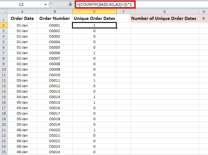
Now lets apply a filter to this range and see the outcome in cell H1. For the purpose of this example, I will deselect order dates belonging to January 1st, 2nd and 3rd in the filter.  
Picture
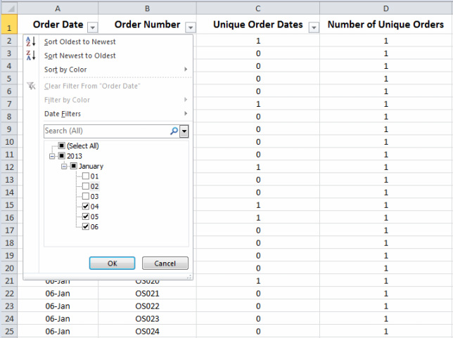
As could be observed in the screenshot below, the value in cell H1 does not represent the correct sum of unique order dates of the data displayed, rather it represents the sum of all values originally selected before applying the filter.
Picture
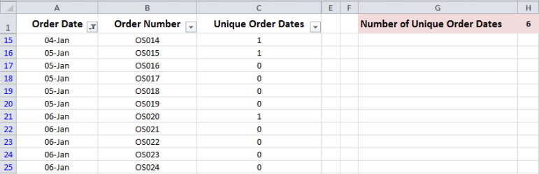
In order to Modify our formula to represent the filtered values, the steps below must be undertaken: 
First, we must create an additional column (column D) in which the SUBTOTAL formula has to be applied to the order numbers (to be applied to the entire range. i.e. from D2 to D25). This column is necessary for the next step as it will help identify those cells which were suppressed through the filter selection. Click here if you want to learn more about the SUBTOTAL formula in MS Excel.
Picture
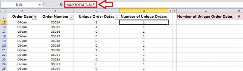
Second, we must create a second tab on the spreadsheet (i.e. Tab2). This new tab will contain two columns. 
  • The first column will identify and list the Order Numbers displayed (and those suppressed) as a result of the filter being applied to the original data on the first tab of the spreadsheet (i.e. Tab1). See the screenshot to the left for the formula used to populate this column. This formula identifies the cells that had been suppressed due to the filter selection. the suppressed cells are represented with "-".
  • The second column identifies the Unique Order Numbers which are displayed after the filter has been applied to the original data on the first tab of the spreadsheet (i.e. Tab1). see the screenshot to the right for the formula used to populate this column. This formula identifies the unique and non-suppressed order numbers with the number "1".
Picture
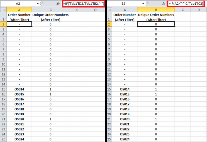
Last but not least, I will go to the original tab (i.e. Tab1) in the spreadsheet and revise the formula in cell H1 to represent the unique order numbers depicted in tab2 of the spreadsheet. By entering this formula, the value in cell H1 will represent the sum of those unique order numbers which have been displayed after applying the filter and the suppressed cells will no longer be counted.
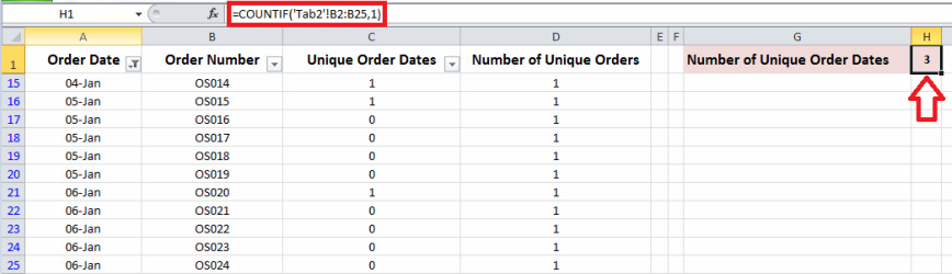
Picture
1 Comment
Soup Accessories link
5/13/2023 12:32:33 am

Thank you foor sharing

Reply


Leave a Reply.

    Categories

    All
    BI
    EXCEL
    MISC
    SQL

    Archives

    June 2020
    May 2020
    April 2020
    March 2020
    February 2020
    December 2019
    November 2019
    October 2019
    September 2019
    August 2019
    July 2019
    June 2019
    May 2019
    April 2019
    March 2019
    February 2019
    January 2019
    December 2018
    November 2018
    October 2018
    September 2018
    August 2018
    July 2018
    June 2018
    May 2018
    April 2018
    March 2018
    September 2017
    August 2017
    July 2017
    June 2017
    May 2017
    April 2017
    March 2017
    February 2017
    January 2017
    December 2016
    November 2016
    October 2016
    September 2016
    August 2016
    July 2016
    June 2016
    May 2016
    April 2016
    March 2016
    February 2016
    May 2015
    April 2015
    March 2015
    February 2015
    January 2015
    December 2014
    November 2014
    October 2014
    September 2014
    August 2014
    April 2014
    March 2014
    February 2014
    January 2014
    December 2013
    November 2013

Powered by Create your own unique website with customizable templates.
  • BLOG
    • Blog Guide
    • Blog History
  • EXCEL
    • Functions & Formulas
    • VBA & Macros
    • VLOOKUP
    • Pivot Tables
    • Conditional Formatting
    • Tricks & Shortcuts
  • BI
    • SAP BOBJ/BW
    • Tableau
  • SQL
  • ABOUT
    • About WBD
    • About Me