Create a dynamic pie chart in MS Excel

---

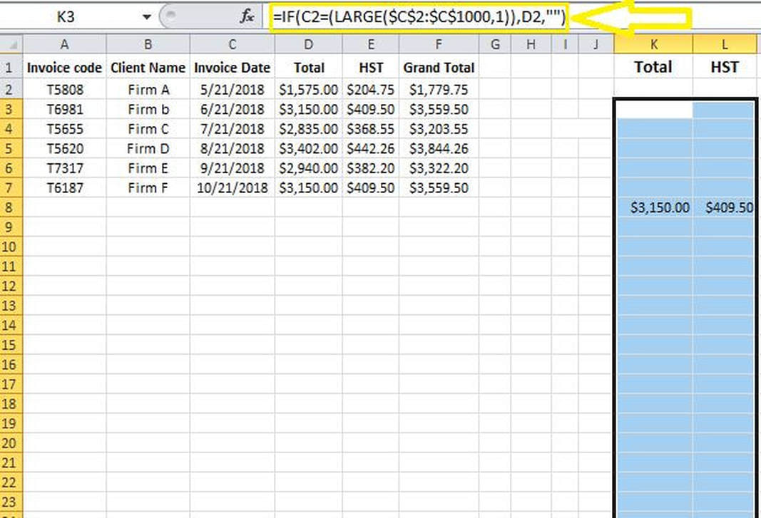
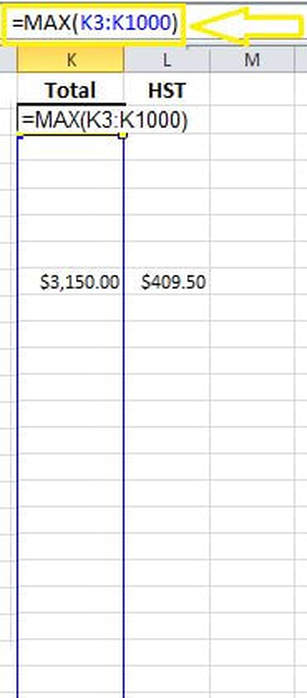
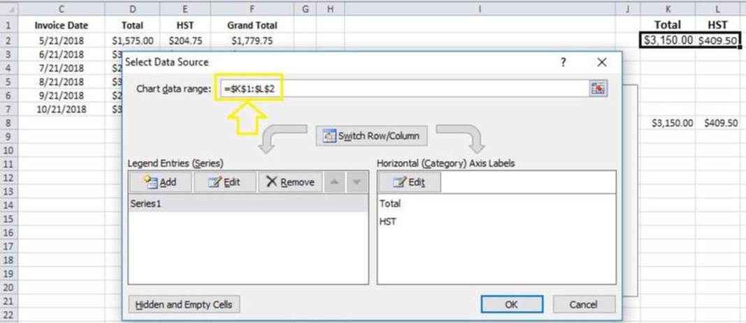
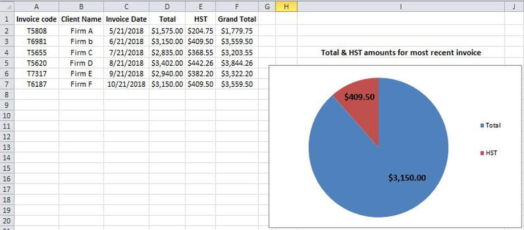
Most of us have experience with creating pie charts in MS Excel and we know how to assign a data range to a pie chart. If the pie chart depends on most recent data entries that would create a requirement to constantly change the data source. For that reason, today I will demonstrate how to create a pie chart that will demonstrate the most recent data entries without needing to constantly change the data source.
​
Take the data set below into consideration

​Say we want to create a pie chart that captures the total invoice and HST amount for the most recent invoice. Doing so is fairly easy. All we have to do is select the most recent data entries as the data source (I.e. in this case cells D7 and E7). But the issue is that as time passes by new data entries are to be inputted into this data set rendering the pie chart stale dated and inaccurate. Here is the solution to this issue.
 
STEP 1] chose two helper columns. In this case I have chosen columns K and L. In the first row of the two columns type the field names (i.e. “Total” and “HST”).

​STEP 2] Leave the second row (i.e. Cells K2 and L2) empty (for now) and starting from row 3 (i.e. cells K3 and L3) enter a formula similar to the one below:

=IF(C2=(LARGE($C$2:$C$1000,1)),D2,"")

Change the cell reference (i.e. change D2 to E2) for the second column. Drag the two formulas down to the lowest point in the spreadsheet that you think data will be generated. 

​These two formulas will display the “Total” and “HST” amounts only for the largest (i.e. most recent) date in the data set. Therefore, as new data is inputted within the original data set, the two helper columns will only display the records for the most recent transaction and the remaining fields will display blank as shown above.
 
STEP 3] Input the following formula in row #2 (which we intentionally left blank in the previous step).

=MAX(K3:K1000) 

STEP 4] create a pie chart and indicate the second row (i.e. cells K2 and L2) of the two helper columns as the data source 

​The pie chart will now always display the most recent data entries based on the invoice date.

---