How to capture the name of a MS Excel worksheet tab in any given cell

---

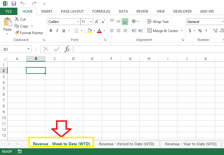
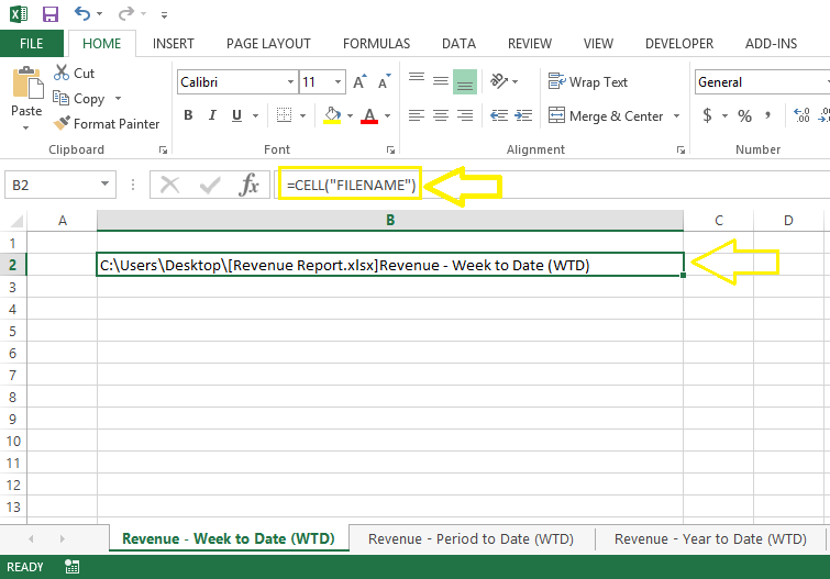
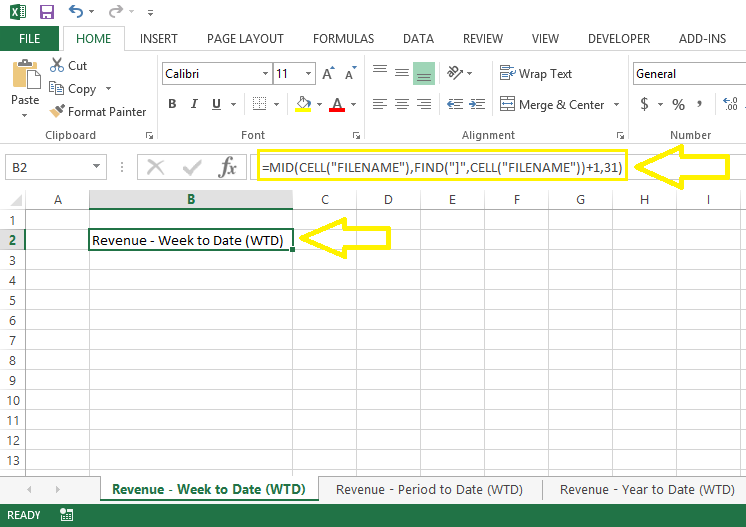
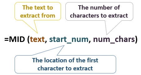
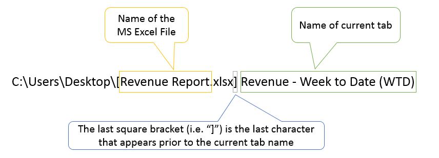
Many MS Excel users work with spreadsheets which contain multiple tabs with unique names. While the name of each tab is represented in the bottom of the sheet, some spreadsheets and business reports require the name of each spreadsheet to appear in the header as well.  

In this blog post I will illustrate how to automatically return the name of Excel tabs in any cell without needing to retype the name manually in that cell.  
​
Consider the spreadsheet below containing three tabs (i.e. “Revenue - Week to Date (WTD)”, “Revenue - Period to Date (WTD)”, and “Revenue - Year to Date (WTD)”)

Let’s say we need to enter the name of each tab at top of the spreadsheet as its header. Here are the steps for doing so.
 
STEP 1]  Insert the following formula in the desired cell                            =CELL(“FILENAME”)
​
This formula will return the full directory of the spreadsheet on your hard drive (i.e. in the case of this example, on my desktop) and it includes the name of the tab (i.e. Revenue – Week to Date(WTD)) at the tail-end as could be seen in the screenshot below: 

STEP 2] If you only want the name of the tab and not the full directory, this could be achieved by using the “MID” and “FIND” functions together in the formula below:
​
=MID(CELL(“FILENAME”), FIND(“]”,CELL(“FILENAME”))+1, 31)

How this formula works?
​
This formula will return only the name of the current spreadsheet tab at the tail-end and not the full directory. The formula begins with the MID statement which returns a specified number of characters in a text string and consists of three main arguments:

The first part of this argument, i.e. CELL (“FILENAME”), determines the text to extract, which is the full file path.

The second part of the argument, i.e. FIND (“]”CELL (“FILENAME”)) +1, extracts everything after the last square bracket (i.e. “]”) symbol.
​
The Find statement locates the position of the first instance of a particular character within a text string. The text character that we are seeking within the directory name is the “]” symbol because the name of the excel file is contained within double brackets which is immediately followed by the name of the particular tab. 

​The third part of the formula, i.e. 31, is the number of characters to be extracted and the reason the number 31 has been chosen is that the name of a tab can NOT be longer than 31 characters in MS Excel, so the maximum character length is chosen. 
 
Advantages of this approach:
1. enables inputting headers without needing to type them manually
2. If the name of a tab is changed/edited, the header will automatically be changed without needing to change it manually
3. Allows us to link the name of a tab to a particular cell to be used in other formulas or be utilized in tasks such as creating dynamic tables

---