How to find cells that contain all of many words

---

Many MS Excel users find themselves in situations where they need to look for certain words or terminology within large spreadsheets which often contain large volumes of text. The Find function (I.e. CTRL+F) enables us to search for certain words, but what if we are seeking cells which contain multiple keywords:
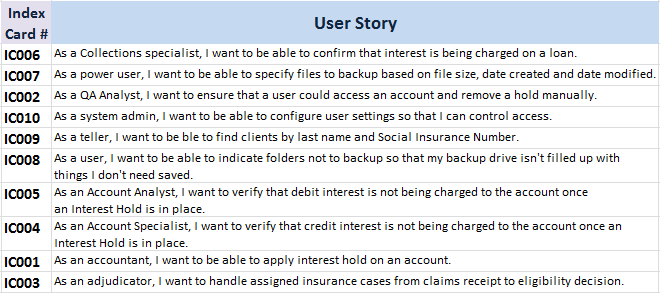
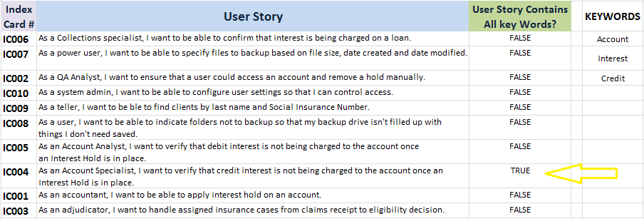
Consider the table below, containing a series of User Stories: 

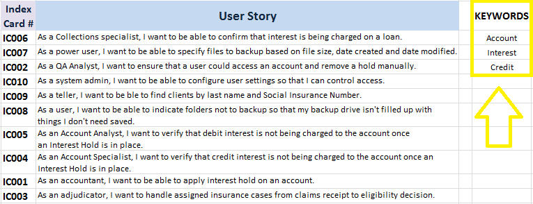
Say we want to find cells that CONTAIN ALL of the three following ​words:

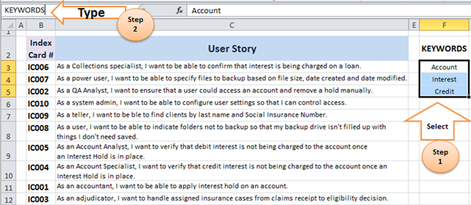
1. Account
2. Interest
3. Credit

Following the steps below will enable us to create a new field that indicates whether or not each cell contains all three key words:
​
STEP 1] Type the key words anywhere in the spread sheet (or in a separate tab if you prefer). 

STEP 2] create a dynamic table for the three key words. I will name the dynamic table “KEYWORDS” (Note: The name cannot contain any spaces).

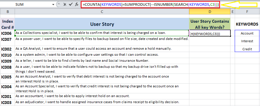
STEP 3] Insert a formula similar to the one below in a separate column. E.g. in this case in column D titled” “User Story Contains all key Words?”

= COUNTA(KEYWORDS)=SUMPRODUCT(--ISNUMBER(SEARCH(KEYWORDS,C3)))

How this formula works?
This formula contains two equations, if the output from these two equations is the same the formula will return “True”, otherwise “False” will be returned. 

The left hand side equation is: COUNTA(KEYWORDS)
The right hand side equation is: SUMPRODUCT(--ISNUMBER(SEARCH(KEYWORDS,C3)))

The left hand side argument in the equation above (i.e. COUNTA(KEYWORDS), counts the number of non-empty cells in the dynamic table (i.e. cells in the F3:F5 range)

The right hand side argument, I.e. SUMPRODUCT(--ISNUMBER(SEARCH(KEYWORDS,C3))), is a bit more complex. First it searches for the three words within the KEYWORDS dynamic table. i.e. SEARCH(KEYWORDS,C3), then the “--ISNUMBER” function checks if a value retrieved from the search is a number or not.

Note] The double dash (--) placed before ISNUMBER is called a double unary operator, and it is used to convert non-numeric boolean values (TRUE / FALSE) into binary values (i.e. 1 and 0) that an Excel array function can understand.
​
​Finally the SUMPRODUCT counts the number of numeric items the “--ISNUMBER(SEARCH(KEYWORDS,C3))” argument.

STEP 4] do an auto fill and apply the formula to the entire data range. Here is the final outcome. As you could see only one of the cells contains all three key words and that cell is indicated with the “True” value in column D.

---