How to highlight the rows whenever cell values change in a data set

---

In one of my previous blog posts I demonstrated how to Replace duplicate values in a column with blank cells. Today, I want to demonstrate how to highlights a row whenever a cell value changes in a dataset using conditional formatting. This is going to be similar to creating a break for knowing when the value in a column changes.
 
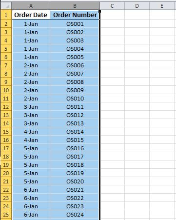
STEP 1] Select the data range.

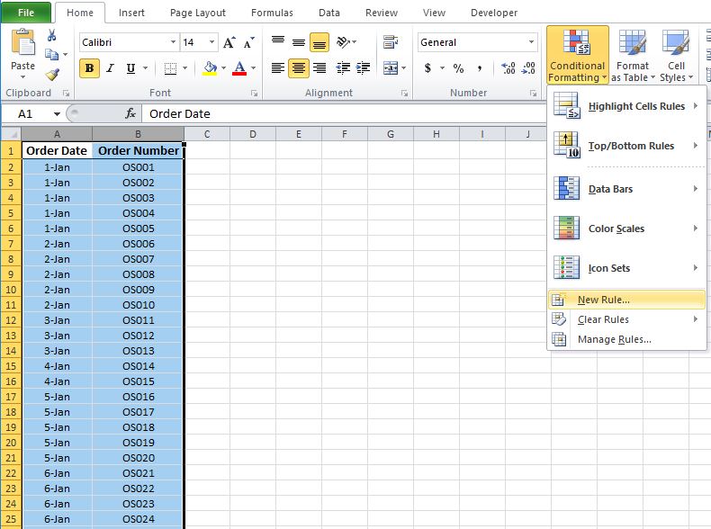
STEP 2] Go to “Conditional Formatting” in the “Home” tab and select “New Rule”.

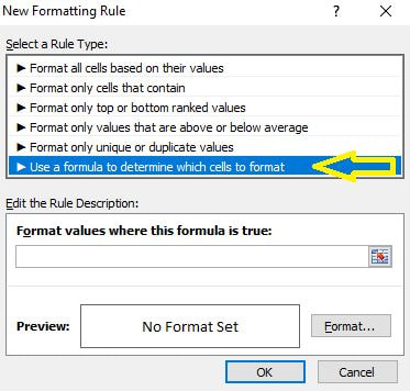
STEP 3] Select “Use a formula to determine which cells to format” in the “New Formatting Rule” page.

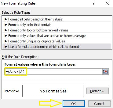
STEP 4] Input the following formula:
=$A1<>$A2

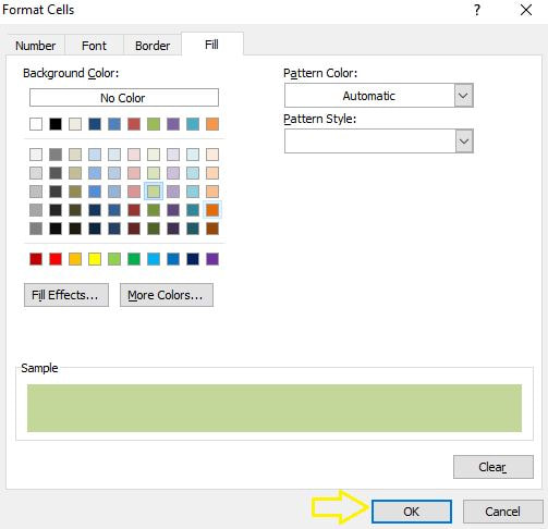
STEP 5] Go to "Format" and select your desired color in the “Fill” tab

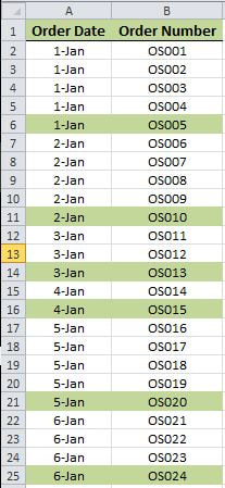
STEP 6] Click "OK" twice. Here is the final desired outcome.

---