Highlight alternating grouping of data in Excel - taking into account blanks (method#2)

---

Two weeks ago, I demonstrated how to highlight alternate data groupings in MS Excel. Last week, I explained how to address blank cells when performing the aforementioned task. It appears that there are still some shortcomings with the method I introduced last week as some overlaps occur depending on the positioning of the blank values within the data set. This week, I will demonstrate a more succinct method for highlighting alternate data groupings taking blanks into account.

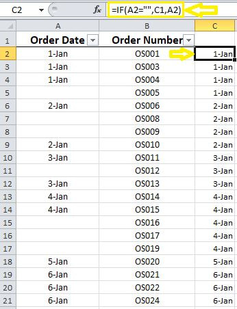
STEP 1] Create a helper column containing the following formula:

                                        =IF(A2="",C1,A2)

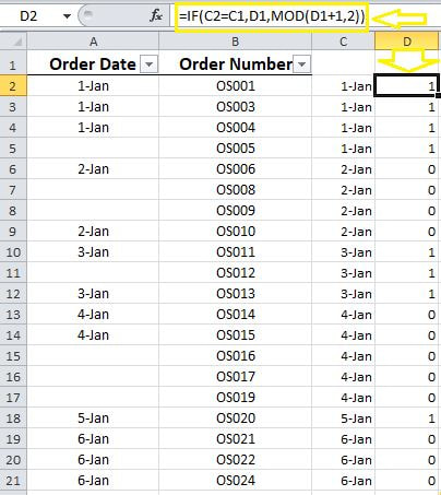
STEP 2] Create a second helper column containing the following formula: 
                                                   =IF(C2=C1,D1,MOD(D1+1,2))

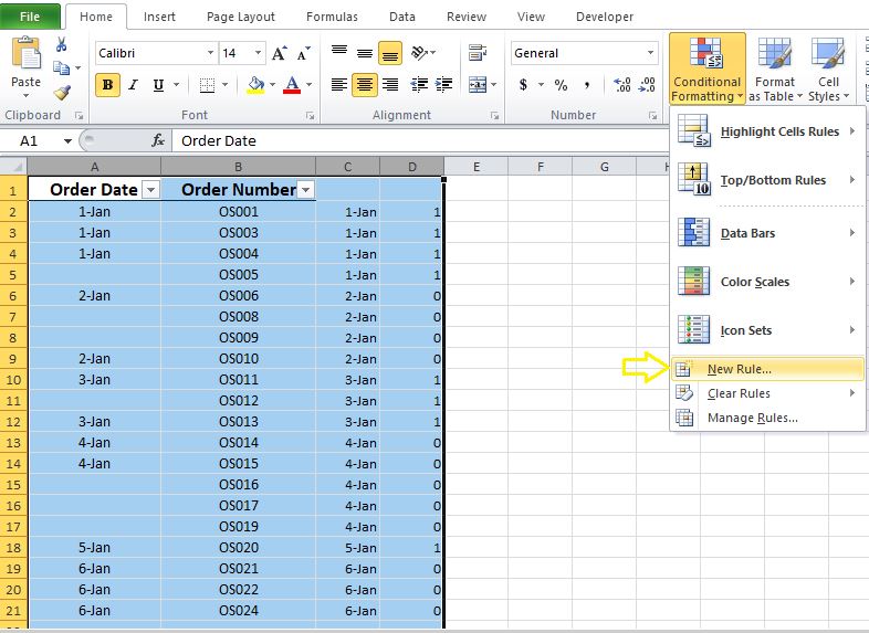
STEP 3] Select the data range and go to “Home”> “Conditional Formatting”>”New Rule”.

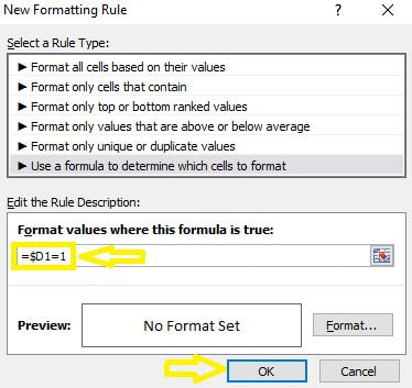
STEP 4] Type in the following formula:
                                                                            =$D1=1

Note] Make sure to reference the empty cell above the first row in which the formula has been inserted, otherwise; the formatting will not be accurate.

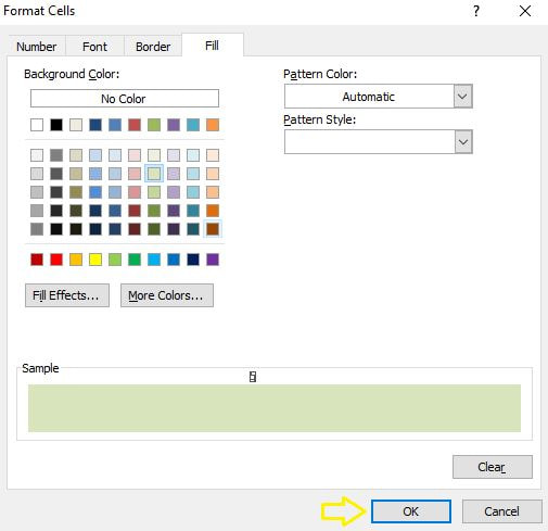
STEP 5] Go to format and select your desired color in the “Fill” tab.

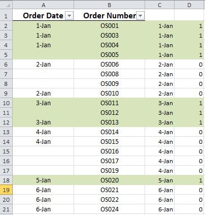
STEP 6] Click “OK” twice. Here is the desired outcome.

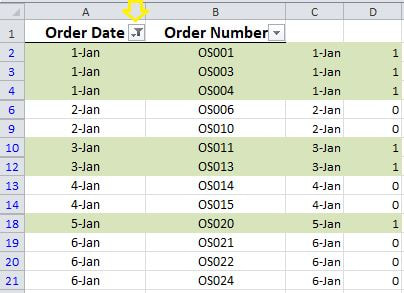
Now I will filter out the blanks.

Mission Accomplished!

---