Replacing Duplicate Values in a Column with Blank Cells in MS Excel

12/20/2013

Say you have a a huge spreadsheet containing one or multiple columns and you want to suppress duplicating values in a given column and replace those values with blank cells. This can be done using the formula below:

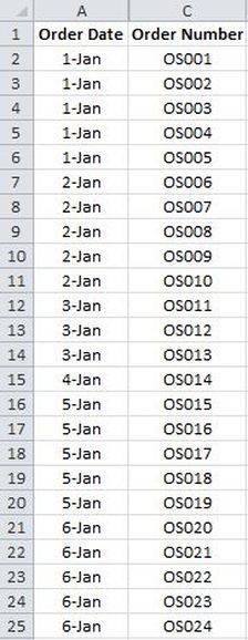
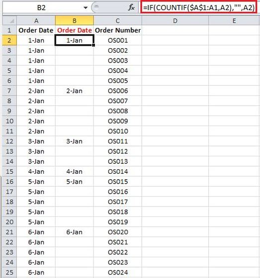
=IF(COUNTIF($A$1:A1,A2),"",A2)

Explanation:
This formula functions by comparing cells with the subsequent cell and wherever a similarity is spotted a blank cell will be displayed, otherwise the subsequent dissimilar cell will be displayed. In this formula, the nested COUNTIF statement is used in order to count the number of repeat cells, and wherever this number is equal to zero a value will be displayed.

To demonstrate further, consider the example of a spreadsheet which contains "Order Dates" and "Order Numbers" where repeating "Order Dates" are prevalent. See the table below:

In order to replace the duplicating values (i.e.Order Dates) with blank cells, I added an addition column (i.e. column B) for Order Date, and I inputted the aforementioned formula in Cell B2. Afterwards, I applied the formula to the entire range by dragging it down. By doing so the repeating values are only being displayed once.

Note: you must have a header for your data otherwise the first value (i.e. cell B2) will also be left blank.

5 Comments

Harry

12/22/2016 08:42:15 pm

Thank you man, this saved my day!

Mehran

12/22/2016 11:13:24 pm

Hi Harry,

You're welcome. I am happy that you found this blog post useful. Stay connected as I will be sharing many many more awesome Excel tips in 2017.

Cheers, Mehran!

susmitha vangala

2/20/2017 08:02:04 am

I am not getting the result by this
after writing the formula in B2
do i need to drag the A,B columns?

Mehran link

2/20/2017 12:39:45 pm

Hi Susmitha,

Thanks for the comment. I don’t quite understand what you mean by “…drag the A,B columns?”. Two things that I predict may be causing your issue are:

First: Do you heave proper headers in A1 and B1?
Second: Have correctly reference locked the $A$1 field as depicted? (i.e. It should be: =IF(COUNTIF($A$1:A1,A2),””,A2)

I hope this helps. Let me know if you have further questions or need more clarification.

Cheers,
Mehran

Frances

3/14/2018 12:57:33 pm

I could not get this to work at first, but when I changed it to

=IF(COUNTIF($A$1:A1,A2)=1,A2,"") it did work.

Thanks for this tip - very helpful!

Replacing Duplicate Values in a Column with Blank Cells in MS Excel

Leave a Reply.

Categories

Archives