Tricky MS Excel interview Question - Conditional IF statement

---

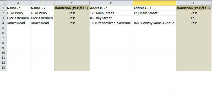
Few months ago I was asked to solve an Excel problem during a job interview.  While the solution seemed to be simple at first glance, the question was a loaded one and took me some time to figure out the answer (I eventually got it right). Here is what the spreadsheet looked like:

It contained 6 columns and three rows of data. The ask was to create a formula in the 7th column  (i.e. column G) that would return “Pass” ONLY when the values in columns C and F were BOTH equal to “Pass” and return “Fail” if otherwise. I initially attempted using the formula below :

=IF(AND(C2="Pass",F2="Pass"),"Pass","Fail")

But this formula kept on returning the “#N/A” error!!!  

After more contemplation, I noticed that the reason for the “#N/A” error is that the values in columns C and F were themselves the result of a formula which used the values in columns A, B, and D, E respectively. For example:

=IF((TRIM(A2)<>TRIM(B2)),"Fail","Pass")

Moreover, the values in columns A, B, D and E were also themselves the results of a VLOOKUP from different tabs. All of this cross-referencing causes some confusions for EXCEL resulting in the #N/A output showing up for the IF statement. As such, my IF(AND formula was not functioning as intended when I referenced columns C and F directly.

The solution is to input the formula used in columns C and F within the IF statement and to use an IF(OR formula instead of an IF(AND formula as shown below:
​
=IF(OR((TRIM(A2)<>TRIM(B2)),(TRIM(D2)<>TRIM(E2))),"Fail","Pass")

​This formula performs the same calculations as in columns C and F and therefore directly references columns A, B, D and E and as such it returns the desired values as shown below

---