|
Every once in a while either myself or a colleague experiences problems with their VLOOKUP formula in MS Excel. The VLOOKUP would not indicate the similar values between the list index and the source and would only return #N/A outputs while similar values do indeed exist between the two lists.
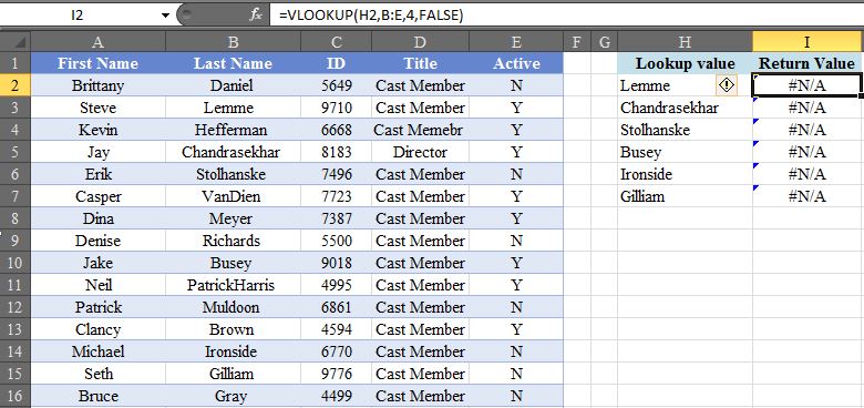
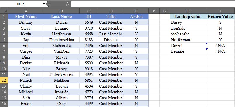
I have been able to diagnose the most common reasons for these anomalies based on my own analysis and also research on the web. Here are three solutions for fixing problems associated with VLOOKUP. I have listed them in order of importance: 1. Replace Extra Spaces with "No Space" In the screenshot below, the "Last Name" column is the lookup value and the "Active" column is the index. As is evident, the formula is returning #N/A despite the fact that the lookup values are present in the table array.
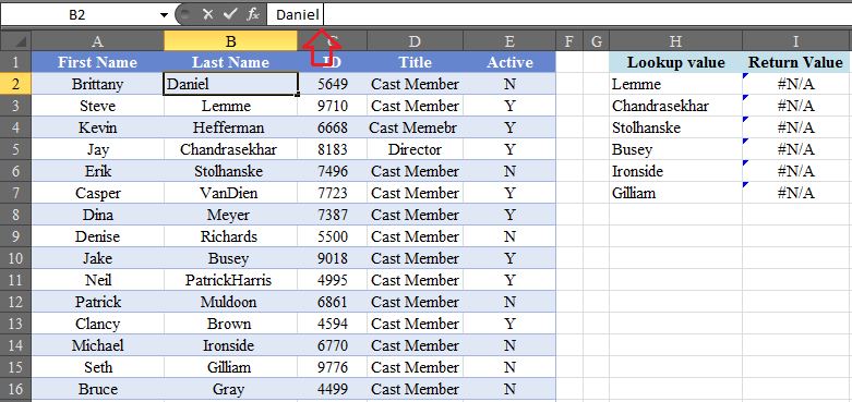
In order to spot the problem, you need to highlight your lookup values and click your cursor past the very end of the entry. Here's the extra space at the end of the input.
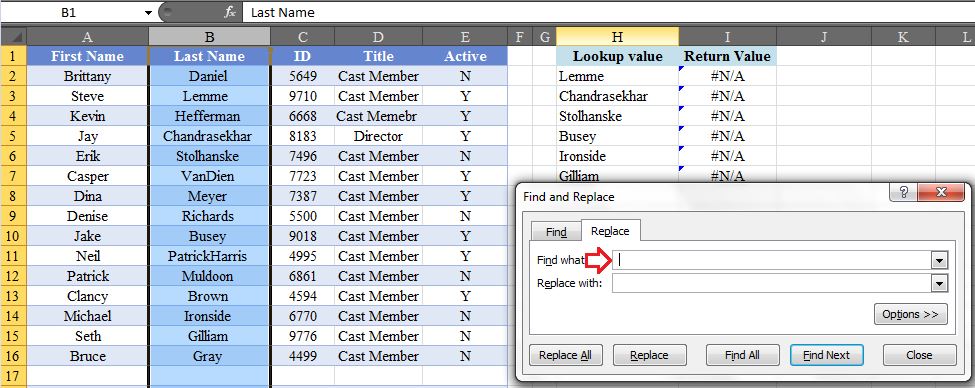
To fix the problem, Click "CTRL+F" and replace spaces with no space in the field that the lookup being done (i.e. Column B). I.e. in the "Find what" section push the space bar button once, and leave the "Replace with" section intact.
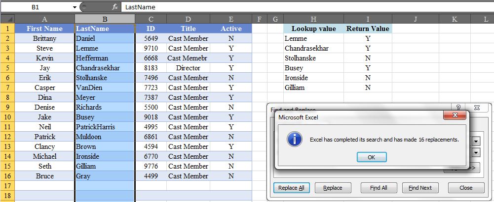
Here is the output :). As you could see the VLOOKUP is now operating correctly as it has identified the Lookup values in the table array.
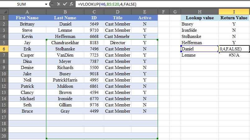
2. Reference Lock Your Array In the screenshot below, the VLOOKUP has not returned any values for the last two lookup values: Daniel, and Lemme.
The screen shot below illustrates the reason for why the VLOOKUP did not pickup the return values for Daniel and Lemme. The reason is simply due to the fact that the table array is not the same across all return value rows.
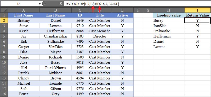
In order to fix this issue all we have to do is to reference lock the table array. This is done by placing dollar ($) signs in the table array range. After placing the dollar signs, as illustrated in the screenshot below, the return values for the VLOOKUP have been corrected accordingly.
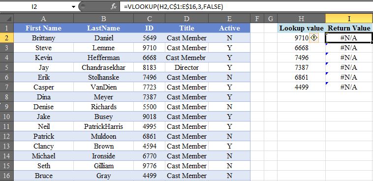
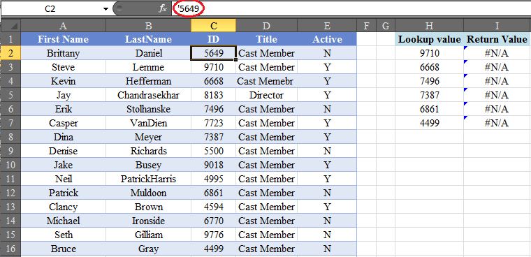
3. Multiply Your Lookup Values by 1 In the screenshot below I have used the values in column C as the lookup values. Notice that these values are numeric. There is a common problem that occurs often when using numeric values as the lookup value in a VLOOKUP. This problem arises when numbers are formatted as text.
Notice the apostrophe before the intended number in the screenshot below. This is due to the way these numbers have been formatted and/or the way they are imported into the spreadsheet.
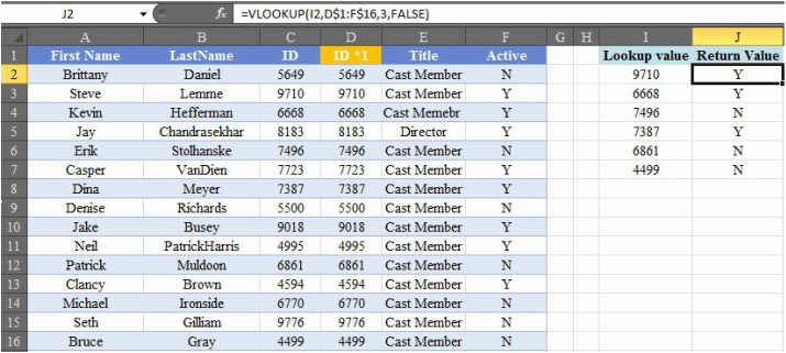
In order to resolve this issue, I have multiplied all values in the ID column (i.e. column C) by 1. the result of the multiplication is inserted in column D in the screenshot below. After performing the multiplication we must also change the table array reference in the VLOOKUP to have it reference the new ID column.
0 Comments
Leave a Reply. |
CategoriesArchives
June 2020
|

