COUNTIF with multiple Criteria – with dynamic references

---

Few weeks ago, I demonstrated how to create a COUNTIF statement with multiple criteria. Click here to view that blog post. This week I want to illustrate the same thing but with dynamic criteria reference values. In my previous blogpost on this topic I introduced the formula below:

=SUM(COUNTIF(B2:B30,{"BARRIE","KINGSTON","BRAMPTON"}))

While this formula works just fine, we will still need to manually input the COUNTIF criteria values (i.e. {"BARRIE","KINGSTON","BRAMPTON"}) within the formula and doing so may become a laborious activity specially if the criteria keeps on changing. With this in mind, inputting the criteria in the form of reference cells instead of actual values will have many advantages such as:

1. If the criteria changes we wouldn't need to manually edit the formula any more
2. Makes the formula significantly shorter
3. Advantageous when we want to use the formula in a Macro (this will be discussed in detail in my next blog post)

​
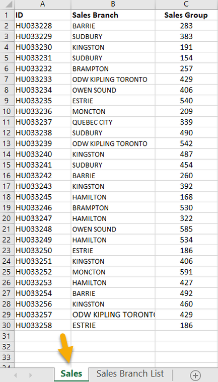
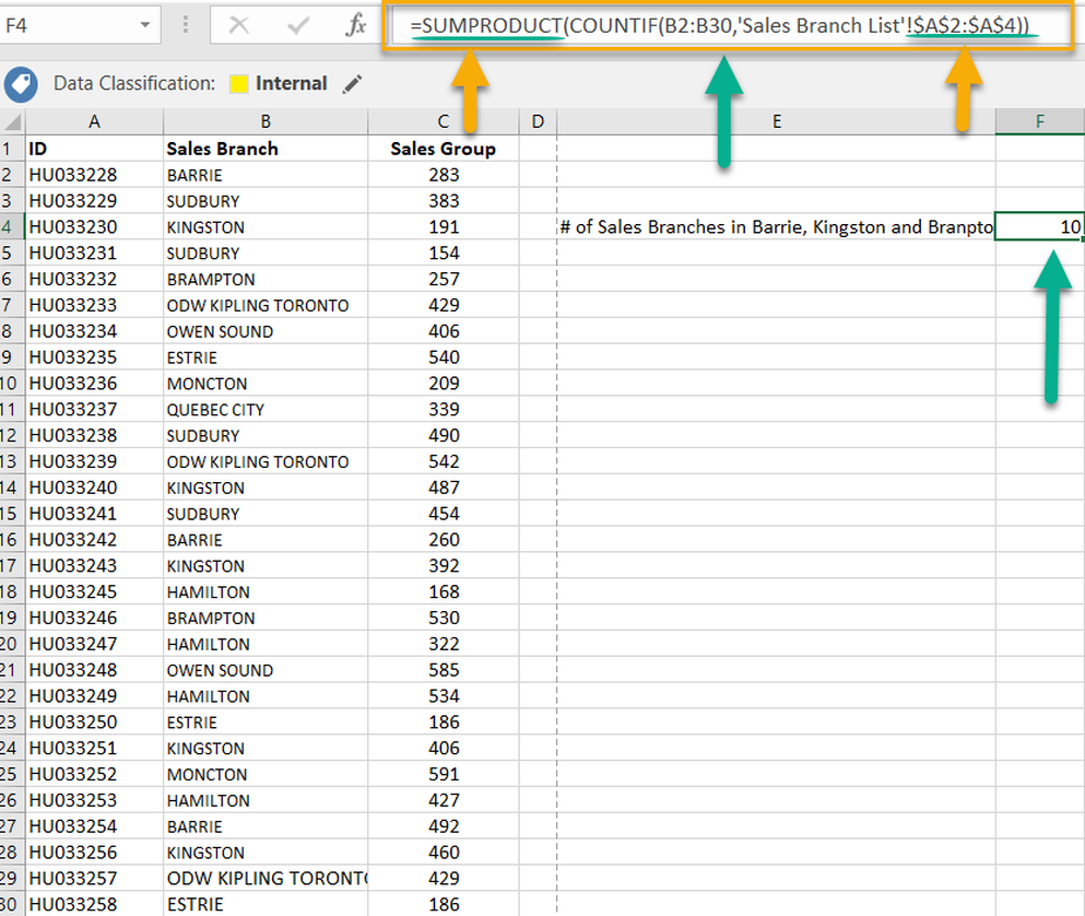
Consider the data set below where the actual data set is stored in the "Sales" tab and the list of desired Sales branches ("BARRIE","KINGSTON","BRAMPTON" stored in cells A2, A3 and A4) are located in a separate tab named "Sales Branch List". 

Here is the generic formula for getting the total number of IDs related to these three sales branches:

=SUMPRODUCT(COUNTIF(B2:B30,'Sales Branch List'!$A$2:$A$4))
​

​​Note that the SUMPRODUCT formula needs to be used instead of SUM and the criteria field (i.e. $A$2:$A$4) needs to be reference locked for this formula to work.

---