How to summarize monthly data into quarters in MS Excel

---

In my last blog post I showed how the OFFSET function can be used to locate a specific cell based on a specified reference point. This week I want to demonstrate how to use the OFFSET function to summarize monthly data into quarters.

The table below contains financial data for twelve months from January to December.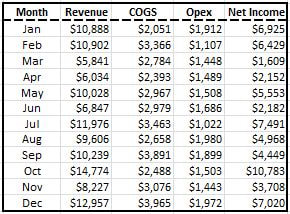

Here is how I will summarize monthly data into quarters:

STEP 1] Form a table containing the four quarters of the year anywhere in the spreadsheet and insert the formula similar to the one depicted below for each of the quarters, starting from Quarter 1, in that table.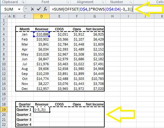

STEP 2] Drag the formula into other cells to cover all four quarter. Make sure to take into account the reference locks (i.e. $ symbols in the formula)

=SUM(OFFSET(D$4,3*ROWS(D$4:D4)-3,,3))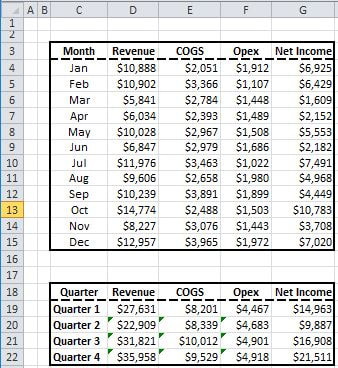

How this formula works:
The formula basically sums the values within the embedded OFFSET formula. In other words, the offset formula (…) returns a grouping of three consecutive cells and the SUM formula adds them up returning the total for the quarter.

As explained din my last blog post the OFFSET formula contains five arguments
                           
                           OFFSET(reference, rows, cols, height, width)

And here is how I’ve applied these three arguments for the formula:

                                  OFFSET(D$4,3*ROWS(D$4:D4)-3,,3))

I have intentionally left the third and fifth arguments blank as they are not needed:

Reference: is cell “D$4”, i.e the first cell that contains data for the first month of the quarter.

Rows: the following formula “3*ROWS(D$4:D4)-3” returns the value for the first row (i.e. January) when calculated for quarter 1. But when we calculate it for quarter 2 (i.e. when the formula dragged down with the reference lock) it will return the fourth tows value (i.e. value for April) for a given column.
Cols: this field is intentionally left blank

Height: we will give the range a height equal to “3” as we want three consecutive months to be referenced.

Width: this field is intentionally left blank
 

---