How to create a dynamic VLOOKUP in MS Excel

​A Dynamic VLOOKUP could be useful for retrieving a select set of fields from multiple tables and/or worksheets. Consider the four tables below containing relevant data for four films: “Mimic”, “Pulp Fiction”, “Scream 2”, and “Spy Kids”. Say we want to write a formula that would retrieve the Director name for each film in a separate table. 

---

Here is the Procedure.
STEP 1] we start off by creating a dynamic table for each of the four tables. This is done by selecting the entire table for each table one at a time, and then typing the name of the particular table in the top left corner name box section. Here is how I did it for the first table (I.e. “Mimic”).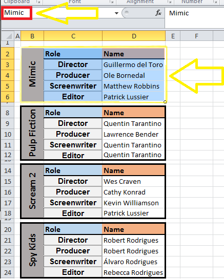

The same thing must be done for the remaining three tables (I.e. “PulpFiction”, “Scream2”, and “SpyKids” as well (IMPORTANT NOTE: No spaces allowed within the name box section).
​
STEP 2] make a new table containing three columns. First column displaying the name of the each table, second column displaying the particular role we want to search by (in this case the “Director”) and a third column is for the VLOOKUP calculation.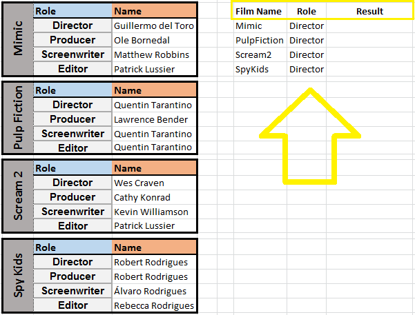

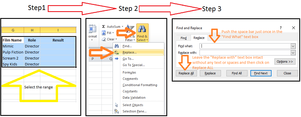
IMPORTANT NOTE: In order for the formula (explained in the following steps) to take effect, there must be no spaces in the film names. Either manually delete the spaces, or use the technique below to have it done very quickly:

​STEP 3] in the result Column input a formula similar to the one below:
=VLOOKUP(H3,INDIRECT(G3),2, FALSE)
 
​​How this formula works? 
This is a simple VLOOKUP but the only difference is that the INDIRECT syntax has been used in the table array part in order to fetch the relevant data from the dynamic tables. The INDIRECT syntax creates a reference from text (in this case from the “Mimic” text in cell G3) and returns a valid reference from that table.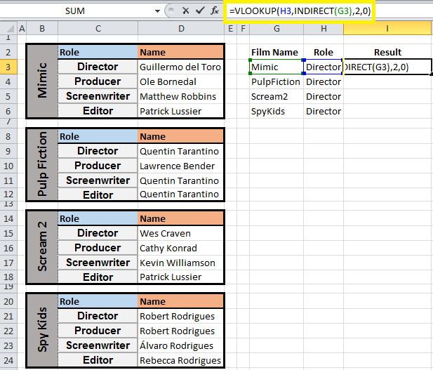

STEP 4] apply the formula to all tables by dragging it down. Here is the final desired outcome.

To look for other unique categories (I.e. Producer, Screenwriter, and Editor) the respective value needs to be inputted in the role column (i.e. Column G).