Highlight alternate data groupings in Ms Excel – Blank Cells Filtered

---

Last week I published a blog post demonstrating how to highlight alternate data groupings in MS Excel. A few viewers have reached out to me since and stated that while the approach did work for them, it causes some overlaps when they filter out blank values in their data set.

 To demonstrate what this means I will use the same data set as last week but will include some blanks in the field in which I want alternating color to be based on.

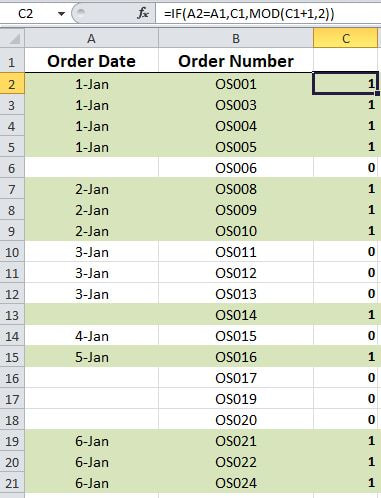
Now I will filter out the blanks.

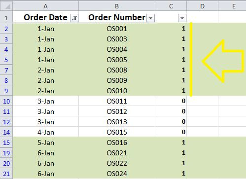
As you could observe in the screenshot above, filtering out the blanks causes two dissimilar groupings to have the same color. This is a result of the blanks having their own unique numbering.

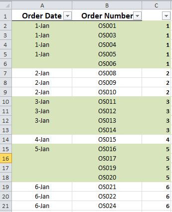
That said, this week I will introduce an alternative and very  creative method for highlighting alternate data groupings that works even after filtering out all blank values.

STEP 1] Replace the formula from last week with the formula below. And apply it to the full column

                    =IF(ISBLANK(A2),C1,IF(A2=A1,C1,C1+1))

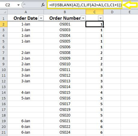
As you could observe in the screenshot above, this new formula does not cause the numbering to change when a blank cell is detected. The numbers get incremented by one if and only if a dissimilar non-blank value is detected in the data set.
 
STEP 2] Select the data range and go to “Home”> “Conditional Formatting”>”New Rule”

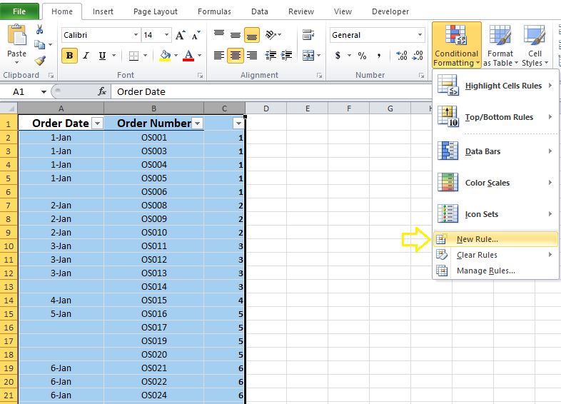
STEP 3] Type in the following formula: 
                                        =ISODD($C1)

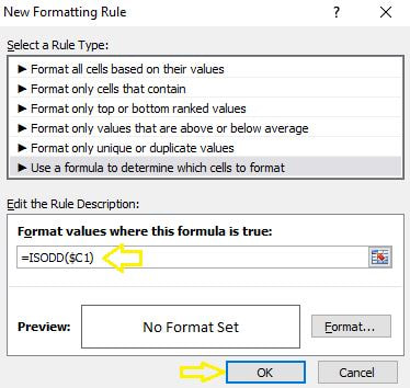
Note] Make sure to reference the empty cell above the first row in which the formula has been inserted, otherwise; the formatting will not be accurate.

STEP 4] Go to format and select your desired color in the “Fill” tab.

STEP 5] Click “OK” twice. Here is the desired outcome.

Now if will filter out the blanks.

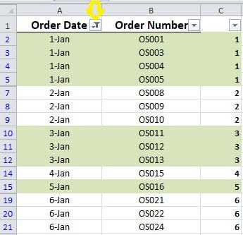
Alternating groupings have been correctly highlighted as desired. This is wonderful :)

---